Space Situational Awareness Software Design

Space situational awareness software tracks every object in Earth orbit — active satellites, spent rocket bodies, debris fragments — and predicts where they'll be in the future. With over 30,000 trackable objects in orbit and that number accelerating with mega-constellation deployments, the software systems that provide SSA are evolving from catalog management tools into real-time operational platforms processing millions of observations daily. Rutagon architects space situational awareness software that handles this scale: ingesting sensor data, maintaining orbital catalogs, computing conjunction assessments, and rendering the orbital environment in real-time visualization.

This article covers the architecture patterns behind modern SSA systems: data ingestion pipelines, orbit determination workflows, conjunction screening at scale, and the visualization layer that makes orbital data actionable for operators and decision-makers.

The SSA Data Pipeline

SSA systems ingest data from multiple sensor types — radar tracking, optical telescopes, laser ranging, and space-based sensors — each with different observation formats, accuracies, and latencies:

┌──────────────┐
│ Radar (S/X)  │──┐
├──────────────┤  │    ┌────────────────┐    ┌──────────────┐
│ Optical      │──┼───▶│ Observation    │───▶│ Orbit        │
├──────────────┤  │    │ Correlation &  │    │ Determination│
│ Laser Range  │──┤    │ Normalization  │    │ Engine       │
├──────────────┤  │    └────────────────┘    └──────┬───────┘
│ Space-Based  │──┘                                 │
└──────────────┘                                    ▼
                                            ┌──────────────┐
                                            │ Object       │
                                            │ Catalog      │
                                            └──────┬───────┘
                                                   │
                                            ┌──────▼───────┐
                                            │ Conjunction   │
                                            │ Screening     │
                                            └──────────────┘

Observation Ingestion

from dataclasses import dataclass
from datetime import datetime
from enum import Enum
from typing import Optional

class SensorType(Enum):
    RADAR = "radar"
    OPTICAL = "optical"
    LASER = "laser"
    SPACE_BASED = "space_based"

@dataclass
class Observation:
    sensor_id: str
    sensor_type: SensorType
    timestamp: datetime
    right_ascension_deg: Optional[float] = None
    declination_deg: Optional[float] = None
    range_km: Optional[float] = None
    azimuth_deg: Optional[float] = None
    elevation_deg: Optional[float] = None
    range_rate_km_s: Optional[float] = None
    sigma_cross_track_km: float = 0.0
    sigma_along_track_km: float = 0.0
    sigma_radial_km: float = 0.0
    correlated_object_id: Optional[str] = None

class ObservationCorrelator:
    def correlate(self, obs: Observation, catalog: dict) -> Optional[str]:
        """Match observation to known catalog object using predicted positions."""
        if obs.correlated_object_id:
            return obs.correlated_object_id

        candidates = []
        for obj_id, state in catalog.items():
            predicted = propagate_to_epoch(state, obs.timestamp)
            residual = compute_residual(obs, predicted)

            if residual < state.correlation_gate:
                candidates.append((obj_id, residual))

        if not candidates:
            return None

        candidates.sort(key=lambda x: x[1])
        return candidates[0][0]

Observation correlation — matching a new radar or optical measurement to a known catalog object — is the first processing step. Uncorrelated observations may represent new objects (launches, breakup debris) or observations with large measurement errors. The correlation gate (maximum acceptable residual) balances detection sensitivity against false correlation rate.

Orbit Determination at Scale

Orbit determination (OD) converts raw observations into orbital state vectors — position and velocity at a reference epoch — with associated uncertainty covariances. For a catalog of 30,000+ objects, OD must run continuously as new observations arrive:

Batch Least Squares for Catalog Maintenance

import numpy as np
from scipy.optimize import least_squares

def batch_orbit_determination(
    observations: list[Observation],
    initial_state: np.ndarray,
    force_model: ForceModel,
) -> tuple[np.ndarray, np.ndarray]:
    """
    Batch least-squares orbit determination.
    Returns refined state vector and covariance matrix.
    """
    def residual_function(state_vector):
        residuals = []
        for obs in observations:
            predicted = force_model.propagate(state_vector, obs.timestamp)
            observed = obs_to_measurement(obs)
            weight = 1.0 / obs.sigma_cross_track_km
            residuals.extend((predicted - observed) * weight)
        return np.array(residuals)

    result = least_squares(
        residual_function,
        initial_state,
        method='lm',
        ftol=1e-10,
        xtol=1e-10,
    )

    jacobian = result.jac
    covariance = np.linalg.inv(jacobian.T @ jacobian)

    return result.x, covariance

The force model includes Earth's gravitational harmonics (typically up to J70x70 for LEO accuracy), atmospheric drag, solar radiation pressure, lunar and solar gravity, and relativistic effects. Getting the force model right determines prediction accuracy, which directly impacts conjunction assessment reliability.

Parallelized Catalog Processing

Processing 30,000 objects requires parallelization. We partition the catalog into independent batches and process them concurrently:

import concurrent.futures
from typing import Callable

def process_catalog_parallel(
    catalog: dict[str, OrbitalState],
    new_observations: dict[str, list[Observation]],
    od_function: Callable,
    max_workers: int = 32,
) -> dict[str, OrbitalState]:
    updated_catalog = {}

    with concurrent.futures.ProcessPoolExecutor(max_workers=max_workers) as executor:
        futures = {}
        for obj_id, state in catalog.items():
            obs = new_observations.get(obj_id, [])
            if obs:
                future = executor.submit(od_function, obs, state.vector, state.force_model)
                futures[future] = obj_id
            else:
                updated_catalog[obj_id] = state

        for future in concurrent.futures.as_completed(futures):
            obj_id = futures[future]
            try:
                new_vector, new_covariance = future.result()
                updated_catalog[obj_id] = OrbitalState(
                    object_id=obj_id,
                    vector=new_vector,
                    covariance=new_covariance,
                    epoch=datetime.utcnow(),
                )
            except Exception as e:
                logger.error(f"OD failed for {obj_id}: {e}")
                updated_catalog[obj_id] = catalog[obj_id]

    return updated_catalog

This architecture mirrors the data analytics pipelines we build for other domains — the patterns of batch processing, parallel execution, and fault-tolerant error handling apply whether the data is orbital elements or financial transactions.

Conjunction Assessment

Conjunction assessment (CA) identifies close approaches between objects and quantifies collision probability. This is the most operationally critical SSA function — a missed conjunction means a potential collision; a false alarm means unnecessary and expensive avoidance maneuvers.

Screening Pipeline

The conjunction screening pipeline operates in two phases:

1. Coarse screening: Fast geometric filters eliminate object pairs that cannot possibly approach within a threshold distance during the screening window (typically 7 days)
2. Fine screening: Precise propagation and probability computation for pairs passing the coarse filter

@dataclass
class ConjunctionEvent:
    primary_id: str
    secondary_id: str
    tca: datetime
    miss_distance_km: float
    radial_miss_km: float
    probability_of_collision: float
    combined_covariance: np.ndarray

def coarse_screen(
    catalog: dict[str, OrbitalState],
    threshold_km: float = 25.0,
    window_days: int = 7,
) -> list[tuple[str, str, datetime]]:
    """
    Filter object pairs using apogee/perigee overlap and
    coplanar geometry. Returns candidate pairs for fine screening.
    """
    candidates = []
    objects = list(catalog.values())

    for i, obj_a in enumerate(objects):
        for obj_b in objects[i + 1:]:
            if obj_a.perigee_km > obj_b.apogee_km + threshold_km:
                continue
            if obj_b.perigee_km > obj_a.apogee_km + threshold_km:
                continue

            raan_diff = abs(obj_a.raan_deg - obj_b.raan_deg) % 360
            if min(raan_diff, 360 - raan_diff) > 15:
                continue

            candidates.append((obj_a.object_id, obj_b.object_id))

    return candidates

def compute_collision_probability(
    primary: OrbitalState,
    secondary: OrbitalState,
    combined_radius_m: float = 20.0,
) -> ConjunctionEvent:
    """
    Compute probability of collision using the 2D Pc method (Alfano/Foster).
    """
    tca, miss_vector = find_tca(primary, secondary)

    combined_cov = primary.covariance[:3, :3] + secondary.covariance[:3, :3]

    rsw_rotation = compute_rsw_rotation(primary, tca)
    projected_cov = rsw_rotation @ combined_cov @ rsw_rotation.T

    cov_2d = projected_cov[1:3, 1:3]
    miss_2d = miss_vector[1:3]

    pc = integrate_gaussian_over_circle(miss_2d, cov_2d, combined_radius_m / 1000)

    return ConjunctionEvent(
        primary_id=primary.object_id,
        secondary_id=secondary.object_id,
        tca=tca,
        miss_distance_km=np.linalg.norm(miss_vector),
        radial_miss_km=miss_vector[0],
        probability_of_collision=pc,
        combined_covariance=combined_cov,
    )

The 2D probability of collision (Pc) method — projecting the encounter into the conjunction plane perpendicular to the relative velocity vector — is the standard approach used by the 18th Space Defense Squadron and commercial SSA providers. The implementation details matter: covariance realism (whether the reported uncertainties actually reflect true prediction errors) determines whether Pc values are meaningful.

This conjunction assessment architecture connects to the broader satellite data processing and AI work we deliver, where the same patterns of high-throughput computation, statistical analysis, and operational alerting apply across space domain applications.

Real-Time Orbital Visualization

SSA data becomes actionable through visualization. Operators need to see the orbital environment — object positions, predicted trajectories, conjunction geometries — rendered in an interactive 3D environment:

WebGL-Based Orbital Display

import * as Cesium from 'cesium';

interface TrackedObject {
  id: string;
  name: string;
  tle_line1: string;
  tle_line2: string;
  object_type: 'payload' | 'rocket_body' | 'debris';
  threat_level: 'none' | 'watch' | 'warning' | 'critical';
}

function renderOrbitVisualization(
  viewer: Cesium.Viewer,
  objects: TrackedObject[],
) {
  for (const obj of objects) {
    const satrec = satellite.twoline2satrec(obj.tle_line1, obj.tle_line2);

    const color = {
      none: Cesium.Color.WHITE.withAlpha(0.3),
      watch: Cesium.Color.YELLOW,
      warning: Cesium.Color.ORANGE,
      critical: Cesium.Color.RED,
    }[obj.threat_level];

    const positions: Cesium.Cartesian3[] = [];
    const now = new Date();
    for (let minutes = 0; minutes < 90; minutes += 0.5) {
      const time = new Date(now.getTime() + minutes * 60000);
      const posVel = satellite.propagate(satrec, time);
      if (posVel.position) {
        const gmst = satellite.gstime(time);
        const geo = satellite.eciToGeodetic(posVel.position, gmst);
        positions.push(Cesium.Cartesian3.fromRadians(
          geo.longitude, geo.latitude, geo.height * 1000
        ));
      }
    }

    viewer.entities.add({
      id: obj.id,
      name: obj.name,
      position: positions[0],
      path: new Cesium.PathGraphics({
        leadTime: 5400,
        trailTime: 0,
        material: new Cesium.ColorMaterialProperty(color),
        width: obj.threat_level === 'critical' ? 3 : 1,
      }),
      point: new Cesium.PointGraphics({
        pixelSize: obj.threat_level === 'none' ? 2 : 6,
        color: color,
      }),
    });
  }
}

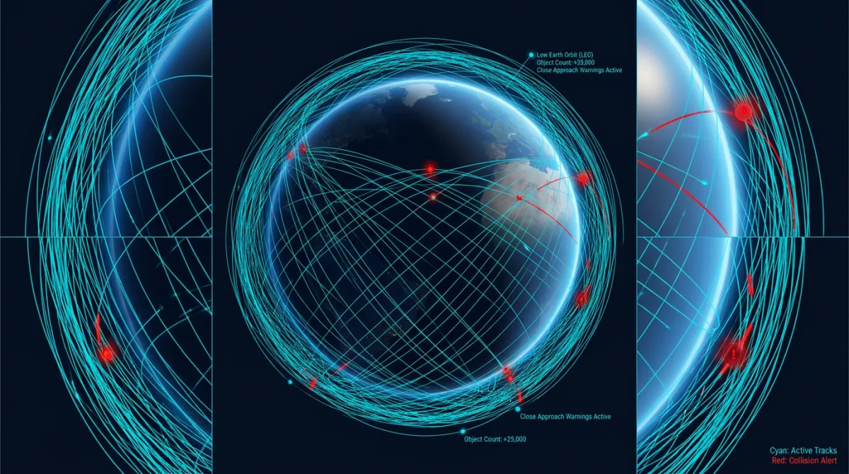
The visualization uses CesiumJS for the 3D globe and orbit rendering, with SGP4 propagation running client-side for smooth real-time updates. Conjunction events are highlighted with connecting lines between threatening object pairs, colored by severity.

For classified environments, the visualization layer deploys to air-gapped networks with no external dependencies — all globe imagery, terrain data, and rendering assets are bundled locally. This deployment model aligns with how we architect solutions for the broader multi-orbit constellation software domain.

Operational Alerting Architecture

SSA systems must generate alerts that reach operators in time to take action. For collision avoidance, that means days of warning for LEO maneuvers and weeks for GEO:

ALERT_THRESHOLDS = {
    "critical": {"pc": 1e-4, "miss_km": 1.0},
    "warning":  {"pc": 1e-5, "miss_km": 5.0},
    "watch":    {"pc": 1e-6, "miss_km": 10.0},
}

def evaluate_alert_level(event: ConjunctionEvent) -> str:
    for level in ["critical", "warning", "watch"]:
        thresholds = ALERT_THRESHOLDS[level]
        if (event.probability_of_collision >= thresholds["pc"]
                or event.miss_distance_km <= thresholds["miss_km"]):
            return level
    return "none"

Alerts route through SNS to email, SMS, and PagerDuty for on-call operators. Critical alerts — Pc above 1e-4 — trigger immediate escalation to the mission director for maneuver planning decisions.

Frequently Asked Questions

How accurate are orbital predictions for conjunction assessment?

Prediction accuracy depends on the object, force model fidelity, and observation freshness. For well-tracked LEO objects with recent observations, position prediction accuracy is typically 50-200 meters over 3 days. For poorly tracked debris with stale observations, errors can reach kilometers. Covariance realism — ensuring the uncertainty estimate matches actual prediction errors — is the critical quality metric for conjunction assessment.

What is the standard for actionable collision probability?

The commonly used threshold for maneuver consideration is Pc = 1e-4 (one in ten thousand). NASA and ESA typically initiate avoidance maneuver planning when Pc exceeds this threshold and the event is within 72 hours. Lower thresholds (1e-5, 1e-6) trigger monitoring and increased observation collection to refine the prediction.

How does SSA handle uncatalogued debris?

Objects too small for routine tracking (1-10cm in LEO) pose a significant collision risk but don't appear in SSA catalogs. SSA systems account for this through statistical flux models — estimating the probability of collision with uncatalogued debris based on orbital altitude, inclination, and known breakup events. Dedicated radar campaigns periodically survey specific orbital regimes to update these statistical models.

Can commercial SSA systems match government tracking capabilities?

Commercial SSA providers (LeoLabs, ExoAnalytic, Numerica) operate growing sensor networks that complement government tracking. In some orbital regimes, commercial systems provide more frequent observations than the Space Surveillance Network. Modern SSA architectures fuse data from multiple providers — government, commercial, and owner-operator — to maximize catalog accuracy and conjunction assessment reliability.

What role does Alaska play in space situational awareness?

Alaska's high latitude provides optimal geometry for tracking objects in polar and sun-synchronous orbits, which include the majority of Earth observation and reconnaissance satellites. Ground-based radar and optical sensors in Alaska see these objects on nearly every orbit, providing the high-cadence observations essential for accurate orbit determination. Alaska is also a prime location for space domain awareness sensors monitoring polar approaches.